CAD Studio - CAD/CAM/GIS/BIM/PLM solutions


")
 2DPlot utility creates algorithmic 2D curves
CADStudio 2DPlot is an AutoLISP utility for AutoCAD - it generates parametric 2D curves (polylines) from mathematic expressions (functions, equations). You can use 2DPlot for educational purposes (math visualization) but also in the design area - e.g. for creation of attractive architectural features, interior design, product design, for DTP (guilloches), for art design, etc. See also 3DPlot for 3D surfaces.
The core application contains functionality required to generate 2D curves from results of math expressions of the type [X,Y] = f(U). You need to specify a user defined function for "f", plus a definition interval of U values (starting value, end value, step size).
After loading 2DPlot you can generate the 2D graphical results simply by calling the LISP function:
(2DPlot functionName startU endU stepU)e.g. (see case 1 - Sinusoid; 100 steps):
(2DPlot fXYt1 (* -2 pi) (* 2 pi) (/ (* 4 pi) 100))The 2DPlot utility also contains several predefined functions (equations of 2D curves) to demo its features. Here is the list of them, including previews of their results:
1) SinusoidA trivial function to demonstrate a simple equation. The math definition used for this function: X=u, Y=sin(u) -- in AutoLISP notation: (defun fXYt1(u)(list u (sin u))) |
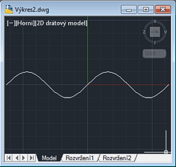 Sinusoid |
2) Damped cosineA combination of multiple curves. The math definition used for this function:
(defun fXYinterf (x / offset)
(defun dampcos (x / dist omag sfreq decfr)
   (setq
     omag  2.0  ; Overall magnitude scale factor
     sfreq 8.0  ; Spatial frequency factor
     decfr 1.5  ; Exponential decay spatial frequency
   )
   (setq dist (sqrt (+ (* x x))))
   (* omag
     (cos (* dist sfreq))
     (exp (- (* decfr dist)))
   )
);defun
  (setq offset 0.9) ; Offset of centres from origin
  (list x (+ (dampcos (- x offset)) (dampcos (+ x offset))))
) |
 Damped cosine |
3) Hypotrochoid 1A roulette traced by a point attached to a smaller circle rolling around the inside of a fixed bigger circle - see Wikipedia. r1 is the smaller radius, r2 is the larger radius, d is the distance of the "pen", th is the current angle from horizontal. The math definition used for this curve: (defun fXYhypotr1 (th / r1 r2) (setq r1 5.0 r2 3.0 d 5.0) ; 3 rotations (list (+ (* (- r1 r2)(cos th)) (* d (cos (* (/ (- r1 r2) r2) th)))) (- (* (- r1 r2)(sin th)) (* d (sin (* (/ (- r1 r2) r2) th)))) ) ) |
 Hypotrochoid 1 |
4) Hypotrochoid 2Another example of the hypotrochoid curve, this time with the parameters of: (setq r1 100.0 r2 2.0 d 80.0) This plot (2000 points) is invoked by: (2DPlot fXYhypotr2 0 (* pi 2) (/ (* 2 pi) 2000.0)) |
 Hypotrochoid 2 |
5) Epitrochoid 1Epitrochoid is similar to hypotrochoid, only the inner circle rolls outside the control circle. This example uses: (setq r1 5.0 r2 2.0 d 2.5) |
 Epitrochoid 1 |
6) Epitrochoid 2You can control the shape and complexity of the curves by changing the parameters of the circles (wheels): (setq r1 5.0 r2 2.25 d 2.5) |
 Epitrochoid 2 |
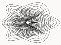
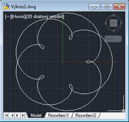
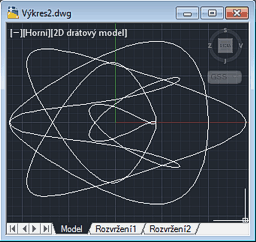
7) Farrel wheelsFarrel wheels is a structure of 3 wheels rolling on each other by the principles of the hypotrochoid. You can specify the size (radius) of all 3 wheels (can also be the same) and their speed (frequency). Farrel wheels are used in a Spirograph or in ancient machines used to generate Guilloches. This particular system uses the following parameters (wheels of the same size):(setq fR1 10.0 fR2 10.0 fR3 10.0) ; radii (setq fn1 13 fn2 -7 fn3 -3) ; speeds (2DPlot fXYfarrel 0.0 1.0 (/ 1.0 1600.0) ) |
 Farrel wheels |
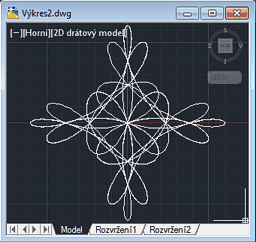
8) Farrel wheels (parametric)The most interesting function - a playground for your own Farrel wheels - specify parameters for the 3 interlocked wheels and watch the results. You can enter the radii for all 3 wheels and their frequency (number of rotations per 0-1 change, can be negative). Try e.g. the parameters (radius+freq):
|
 Farrel wheels (param) |
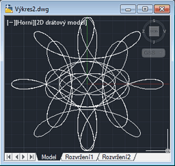
9) GuillocheA combination (superposition) of two hypotrochoids with the parameters of [5 3 5] (with phase offset 1.5x). By combining multiple hypotrochoids or epitrochoids you can generate pleasant and symmetrical curves often used on banknotes, printed stocks, diplomas, etc. |
 Guilloche |
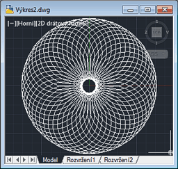
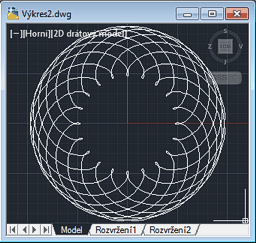
10) Guilloche (parametric)This is a series of guilloche curves from the example above. Each next curve has its parameters scaled down by 10%. |
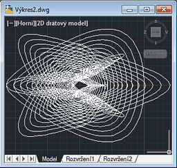 Guilloche (parametric) |
11) Epitrochoid (slow)This is a series of epitrochoids with scaled-down parameters similar to the example above. It uses the epitrochoid from the case #5 but repeats it (and scales to 90%) 10-times. Also uses a different method of plotting the polyline - 2DPlotP. This function plots the curve by calling the PLINE command. |
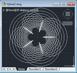 Epitrochoid (param) |
12) Catenary (řetězovka)This is a simple parametric curve defined by: (defun fXYcatenary (x) (defun cosh (x) (/ (1+ (exp (* 2.0 x))) (* 2.0 (exp x)))) (list x (* fCa (cosh (/ x fCa)))) )where fCa is the catenary parameter. |
. |
13) Fermat's spiral (parametric)This is a simple parametric curve defined by: (defun fXYfermat (x) (list (* fCa (sqrt f)(cos f)) (* fCa (sqrt f)(sin f)) ) )where fCa is the spiral step parameter (+/-). |
. |
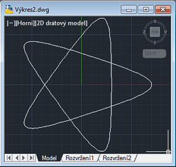
14) Lissajous curveThis is well-known parametric curve defined by: (defun fXYlissajous (f) (setq a 9 b 7 delta (/ pi 2.0)) (list (* 10.0 (sin (+ (* a f) delta))) (* 10.0 (sin (* b f))) ) ) |
. |
15) Nice curveThis is a 6400-nodes long parametric curve defined by (0-2pi): (defun fXYnice (f) (list (* 5.0 (- (cos f) (* (cos (* 80.0 f)) (sin f)) ) ) (* 2.0 (- (* (sin f) 2.0 ) (sin (* 80.0 f)) )) ) ) |
. |
16) CuriousThis is a 1600-nodes long parametric "drunk" curve with a simple definition: (defun fXYcurious (f) (list (+ (sin (* f f)) f) (/ (+ (cos (* f f f)) (* f f)) 5.0) ) ) |
. |

Load the 2DPlot.vlx (or .LSP). If you want to just plot your own function, type or load its definion and call the (2DPlot) function with appropriate parameters. If successful, (2DPlot) returns the number of nodes created. Do not use too detailed (small) step values when testing curve shapes.
If you want to run the demo functions, start 2DPlot by typing the 2DPLOT command. Select the curve you want to generate by typing the respective number. The progressbar informs you about the process of curve generation.
The generated object type is LWPOLYLINE (AcDbPolyline). You can explode it to individual Lines.
If you want to use your own 2D functions in 2DPlot, you need to perform two operations: 1) define the function; 2) call the (2DPlot) function to draw it. E.g. if you want to draw a 2D curve defined by y = sin(x^2), use these two LISP "commands" (e.g. on the AutoCAD commandline):
(defun myFunc (x) (list x (sin (* x x))))
(2DPlot myFunc -2.0 2.0 0.1)
The first one defines a function "myFunc" (needs to return a list of X Y coordinates). The second calls the plot engine for points in the interval (-2;2) in both dimensions, in steps of 0.1.
You can also use equations and expressions based on the polar coordinate system (not cartesian). Just convert the theta/radius polar coordinates to X/Y when returning values from your custom polar function:
(list (* radius (cos theta)) (* radius (sin theta)))An example:
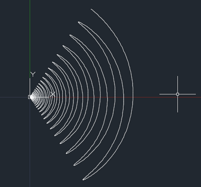
; define polar function "fPolar1" for a range (0-1.5>:
(defun fPolar1 (u / r tau alfa R0)
;x = (* r (cos th))
;y = (* r (sin th))
 (setq r u) ; radius is the driving parameter
 (setq tau 1.1) ; constant - example
 (setq alfa 1.0) ; constant - example
 (setq R0 0.1) ; constant - example
 (setq th (* alfa (sin (/ (* pi (log (/ r R0))) (log tau))))) ; your polar expression
 (list (* r (cos th)) (* r (sin th))) ; return (X Y)
)
Then call (type in):
(2Dplot fPolar1 0.001 1.5 0.001)which will give something like that:
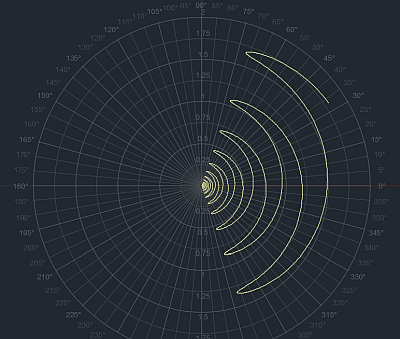
Similar function superimposed on a polar grid from DrGrid:
2Dplot also creates an auxiliary data table after generating a mathematical curve, which can then be drawn (if the AnimDraw library is loaded) as animated - by calling the LISP function (2dplotanim). See the tip and video:
NB:
2DPlot (VLX) is freeware. ARKANCE's customers can download full source version of 2Dplot (.LSP) from the Helpdesk server.
2DPlot is a free utility by CAD Studio (ARKANCE), do not publish it online on other than CADstudio's web servers. Contact ARKANCE for feature enhancements.
 Download the 2DPlot application (for AutoCAD 2017-2026)


